|
Results and discussion
Land cover (LC) of the region is assessed using the preprocessed temporal remote sensing data using Normalized Difference Vegetation Index (NDVI). Figure 3 depicts the vegetation cover based on NDVI for Chennai region during 1991-2012. Table 5 tabulates the vegetation cover dynamics, which show that the percentage of vegetative cover has drastically reduced by 22% during the past two decades, with the increase in non-vegetative area (buildings, open space, water, etc.). As per the LC analysis, the current vegetation cover is about 48.18%. To understand the status of various land use (LU) classes in the region classification of temporal remote sensing data were done using GMLC. LU analysis helps to demarcate the different classes and LC provides only the details of vegetative cover (which might be vegetation and also cropland).
Year |
Vegetation (%) |
Non- vegetation (%) |
1991 |
70.47 |
29.53 |
2000 |
56.7 |
43.27 |
2012 |
48.18 |
51.82 |
Table 5: Vegetation cover changes in Chennai
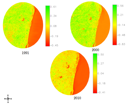
Figure 3: Temporal land cover analysis using NDVI
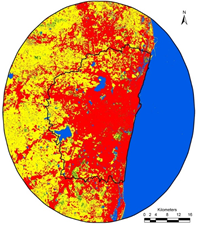
Figure 4 depicts land use changes, based on the analysis of temporal remote sensing data using Gaussian Maximum Likelihood Classifier (GMLC). Table 6 provides land use statistics, which reveals that the area under vegetation declined from 70% to 48% with an increase in urban (paved) surfaces from 1.46% to about 18.5%. Table 7 tabulates overall accuracy and kappa statistics obtained for classified images– these results show that the classified and ground truth data are closely related. Overall accuracy and kappa statistics showed a good relation of the classified data with ground truth data.
Land Use category |
Built-up |
Vegetation |
Water body |
Others |
Area (%) |
Area (%) |
Area (%) |
Area (%) |
1991
2000
2012 |
1.46
2.52
18.55 |
1.38
0.8
1.51 |
27.64
27.25
28.15 |
69.52
68.35
51.38 |
Table 6: Land use in the study region
Figure 4: Output of land use analysis in the study region
Category |
1991 |
2000 |
2012 |
Producer’s
Accuracy |
User’s
Accuracy |
Producer’s
Accuracy |
User’s
Accuracy |
Producer’s
Accuracy |
User’s
Accuracy |
Built-up |
92.04 |
93.02 |
90.42 |
97.38 |
78.23 |
93.02 |
Vegetation |
99.31 |
92.49 |
97.75 |
99.42 |
98.98 |
79.49 |
Water body |
91.50 |
93.84 |
91.65 |
89.52 |
99.47 |
93.84 |
Others |
96.28 |
92.45 |
92.70 |
98.82 |
39.50 |
76.45 |
Overall Accuracy |
92 |
91 |
97 |
Kappa |
0.92 |
0.9 |
0.93 |
Table 7: Accuracy assessment from confusion matrix and kappa statistics
Figure 5 illustrates the urban growth pattern during 1991 to 2012, derived from the classified data
Shannon’s entropy (Hn): Shannon’s entropy aids in assessing the urbanisation pattern and was calculated for each zone considering the gradients and as shown in figure 6. The values closer to 0 indicates of a compact growth, as in 1991. All zones show a compact growth or more concentrated growth towards the central business district as even seen in classified data. The Shannon’s entropy values have increased temporally to 0.4 indicating the tendency of dispersed fragmented growth or sprawl in all directions. This indicates a fragmented outgrowth and mostly in North west direction. Increased patches in all zones indicate that the city is heading towards higher fragmented outgrowth and more clumped inner core. Further this pattern is analysed using landscape metrics for better understanding at each gradient and zone.

Figure 6: Shannon entropy
Analysis of spatial metrics: Results of all metrics are given in fig the X-axis represents the gradients considered and Y-axis, the Metric value.
Percentage of landscape (PLAND): PLAND equals the proportion of landscape comprised of the corresponding class patches. Built up proportion was computed to understand the ratio of built up in the landscape. The results given in Figure 7a, reveal that the proportion has increased during the three decades with the tremendous growth in the central circles. The outer gradients show a slight but significant increase, which indicate sprawling development in the periphery and buffer. The NW shows a relatively higher increase as compared to that in the NE and SW.
Number of patches (NP): NP equals the number of built up patches in a landscape. It indicates the level of fragmentation in built up landscape. Figure 7b depicts the significant increase in number of urban patches during two decades in all directions in all gradients, indicating the fragmentation of landscape during post 2000. Patches at the city centre are combining to for single clumped dominant patch, whereas in outer gradients is more fragmented.
Patch Density (PD): Patch density was computed as an indicator of urban fragmentation. As the number of patches increase, patch density increases representing higher fragmentation. shows the trends in patch density and comparable to the number of urban patches i.e., fragmented urban patches towards the fringes in all directions and a clumped patched growth at the center.
Largest patch index (LPI): Largest Patch Index (LPI) was computed to represent the percentage of landscape that contain largest patch. Figure 7d illustrates that gradients at the center are with higher values due to the larger size urban patches indicating compact growth. The declining trends at the gradients away from the city center at fringes or peri urban areas indicates of fragmented urban patches.
Landscape shape index (LSI) and Normalized landscape shape index (NLSI): Landscape shape index provides a simple measure of class aggregation or disaggregation. Aggregation is measured via class edge. Normalized landscape shape index is similar to landscape shape index but this represents the normalized value. and Figure 7b depicts LSI and NLSI respectively indicate that lower values in the gradients at the city center during post 2000 highlights of simpler shapes with compact urban patches compared to the fringes which show complex shape with the fragmented outgrowth.
Clumpiness (CLUMPY) and Aggregation Index (AI): Clumpiness index represents the status of urban landscape and is the measure of patch aggregation. It measures the clumpiness of the overall urban patches. Clumpiness ranges from -1 to 1 where Clumpy is -1, when the urban patch type is maximally disaggregated, Clumpy is 0 when the patch is distributed randomly and approaches 1 when urban patch type is maximally aggregated. Aggregation Index gives the similar indication as clumpiness i.e., it measures the aggregation of the urban patches, Aggregation index ranges from 0 to 100. An analysis of clumpiness index for the year 1991, explained that the city, except a few patches in the outskirts and buffer, had a simple clumped growth at the center business district with the values close to 0. Analysis for the year 2012 indicated a high fragmented growth or non-clumped growth at outskirts and more clumped growth in the center. The aggregation index showed the similar trend as the clumpiness index.also revealed that the center part of the city is becoming single homogeneous patch whereas the outskirts are growing as fragmented patches of urban area destroying other land uses and forming a single large urban patch.
Patch cohesion index: Figure 7c measures the physical connectedness of the urban patches. Higher cohesion values in 2012 indicate of higher urban patches while lower values (in 1991) illustrate of fewer urban patches in the landscape.
Percentage of Like Adjacencies (PLADJ): This indicates the percentage of cell adjacencies of the corresponding patch type. Figure 7j depicts that the urban patches in the landscape are most adjacent to each other in 2012, and were fragmented in 1991 and 2000. This illustrates that urban land use is dominant in 2012 and is in the process of forming a single patch.
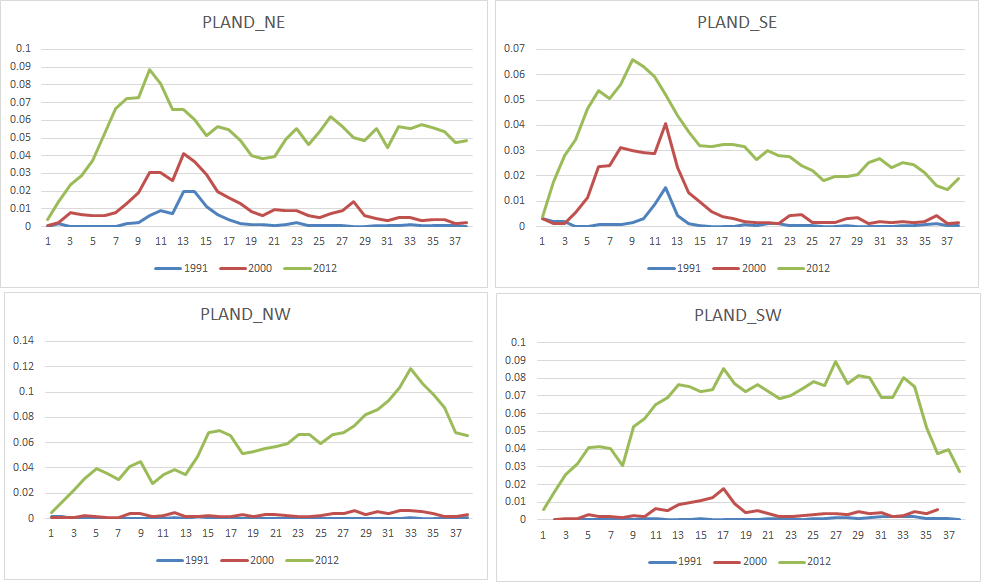 Figure 7a: Percentage of landscape (PLAND) Figure 7a: Percentage of landscape (PLAND)
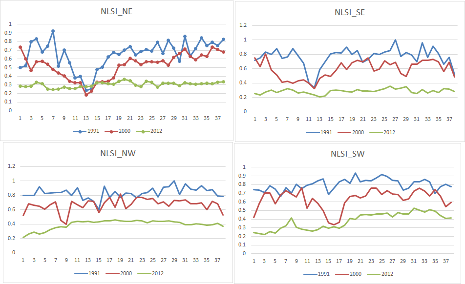
Figure 7b: Normalized Landscape shape index (LSI)
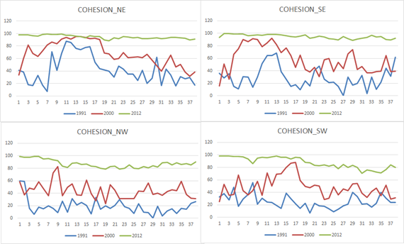
Figure 7i. Patch cohesion index
Visualisation using Fuzzy AHP CA-Markov: Prediction for the year 2026 was performed considering both scenarios and agents as specified earlier. Wherein water bodies and coastal regulation areas were kept constant insisting no development at these areas. Subsequently prediction was done without considering CDP. Table 8 shows % land use category change. Built-up areas have been increased two fold, decrease in vegetation and increase in other categories can be observed from 2013 to 2026. Significant changes can be seen in areas which falls within the CMDA boundary such as Korathur and Cholavaram lake bed, Redhills catchment area, Perungalathur forest area, Sholinganallur wetland area etc. as visualized in figure 9.
Categories / Year |
Predicted 2026 with CDP |
Predicted 2026 without CDP |
Builtup |
36.6 |
36.5 |
Vegetation |
2.4 |
2.4 |
Water |
27.9 |
27.8 |
Others |
33.1 |
33.3 |
Table 8: Predicted land use statistics for the year 2026.
Predicted 2026 with CDP |
Predicted 2026 without CDP |

Figure 9: Predicted land use categories for the year 2026. |